The problem
Classifying skin pathologies from clinical images means asking a model to separate classes that, to the naked eye, look a great deal alike. Two lesions of very different natures can share a shape, a border and a tone; conversely, the same pathology changes appearance with skin tone, lighting and whichever device took the photograph.
On top of that sits the constraint that shapes everything else: clinical datasets are imbalanced. Common cases numerically overwhelm rare ones, and the rare ones are precisely what matters. A model that naively optimises overall accuracy learns very quickly to ignore minority classes - and posts a flattering score that says nothing about how useful it actually is.
Why start from pre-trained models
Training a deep convolutional network from scratch assumes a volume of annotated data that clinical imagery does not provide. Transfer learning works around that: you take a network already trained on a general-purpose corpus, keep the early layers - which learned low-level patterns, edges, textures, gradients, valid well beyond their original domain - and relearn the upper layers on the images you care about.
The remaining choice is how deep to unfreeze: everything frozen except the classification head, or let the last convolutional blocks breathe. The more you unfreeze, the more the model adapts to the domain, and the more it risks overfitting a small dataset. It is a dial to tune, not a box to tick.
EfficientNet against ResNet
Both architectures answer the same question - how do you gain depth without training degrading - in two different ways. ResNet introduces residual connections: each block learns a difference from its input rather than a full transformation, which lets the gradient travel back intact through dozens of layers.
EfficientNet starts from another observation: depth, width and input resolution cannot be tuned independently. Its compound scaling grows them together at a fixed ratio, which yields distinctly leaner models at a comparable parameter budget.
So the comparison is not a matter of which one posts the better score. Under an identical protocol - same data, same augmentations, same unfreezing strategy - it is about behaviour: convergence speed, hyperparameter sensitivity, inference cost, and above all how each holds up on minority classes rather than on the average.
Preprocessing, where it is really decided
Stain normalisation addresses a well-documented nuisance in medical imaging: from one centre to another, from one device to another, the same tissue does not render the same way. Without correction, the network learns the device signature alongside the pathology, and collapses the moment you show it a source it has never seen.
Advanced data augmentation plays on a different register. Rotations, flips, crops, brightness and contrast shifts: the aim is to manufacture plausible variability, the kind you would genuinely meet in a clinical setting, without inventing images no patient would ever produce. On rare classes, augmentation does double duty - it regularises and it rebalances.
Imbalance is handled in parallel, at the sampling level and in the loss function, so that an error on a rare class weighs what it should instead of dissolving into the mass.
What the published model does
The repository publishes where this work landed: a compact CNN - four convolutional blocks followed by five dense layers - trained on HAM10000 and its seven lesion categories, with inputs resized to 28×28. On the evaluation split it reaches 0.99 accuracy and 0.99 macro F1.
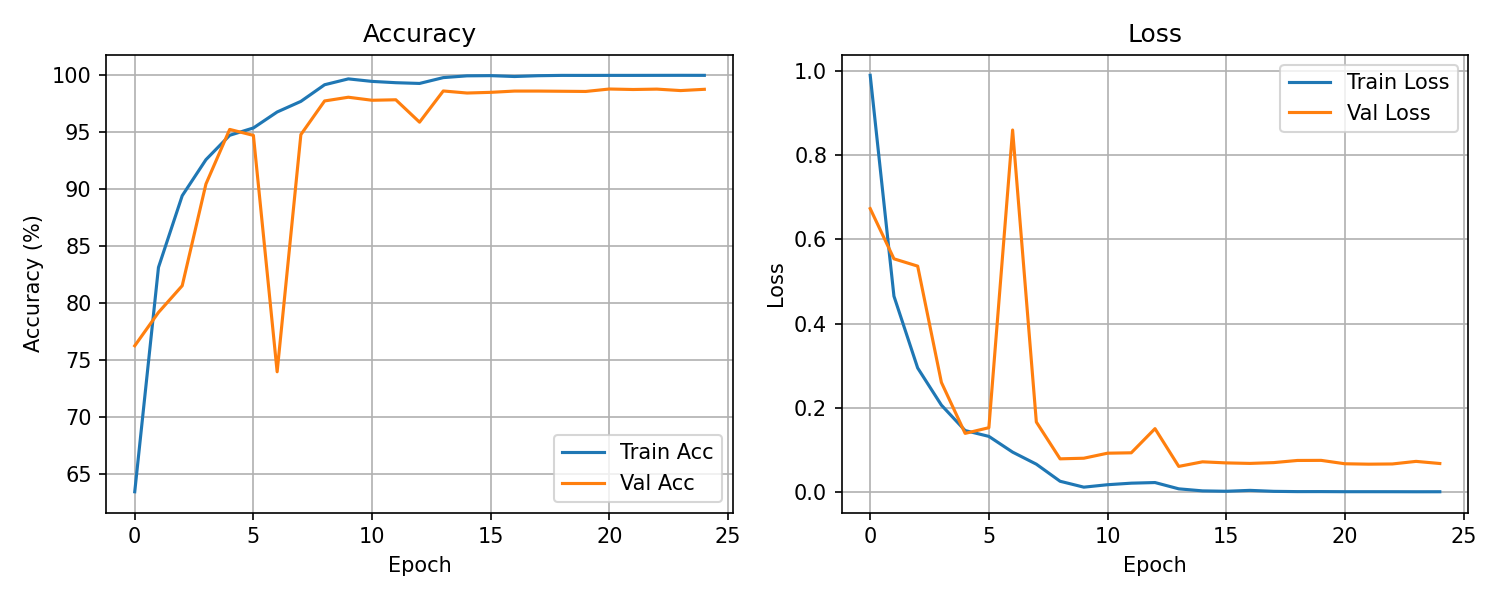
The training curves tell the story better than the final score does. Validation accuracy drops sharply at the sixth epoch - from 95% to 74%, with the matching loss spike - before recovering and settling around 98.7%. An isolated dip of that shape points to a learning rate too aggressive for a rugged loss surface, not to a data problem. The final gap between training and validation, 100% against 98.7%, is the residual overfitting you never fully shake off on a dataset this size.
Where the average lies
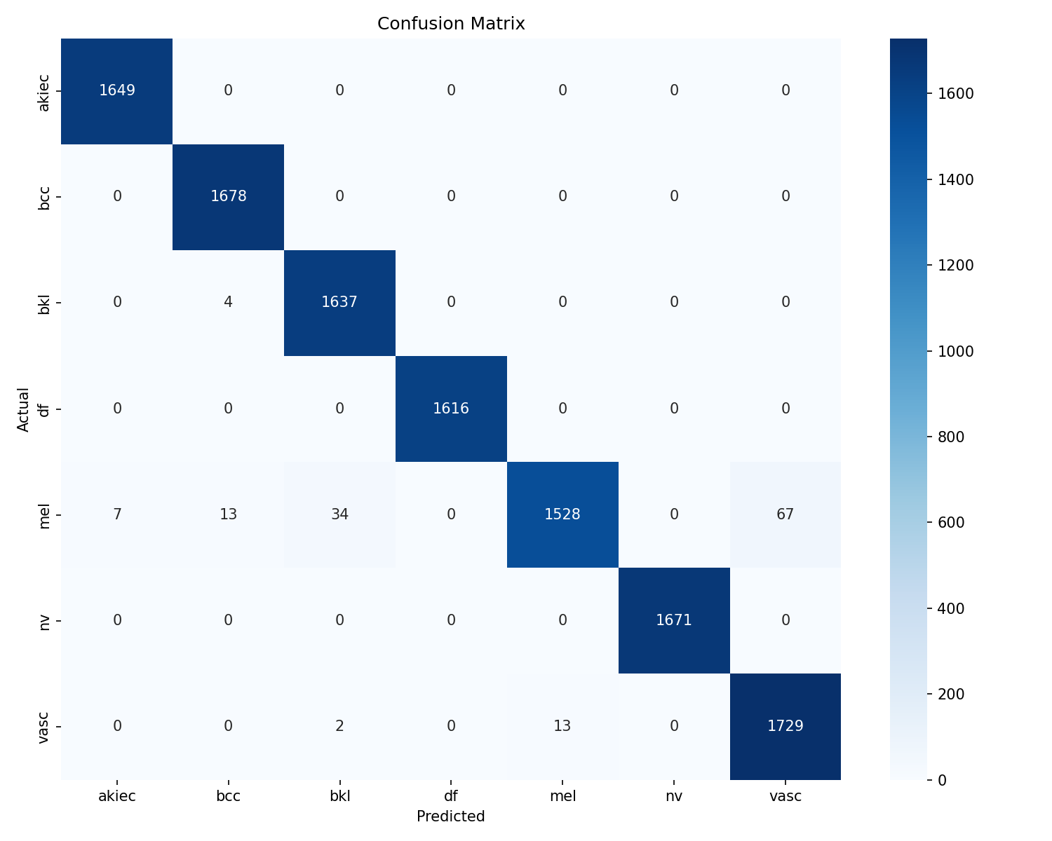
The confusion matrix confirms the methodological point. Six classes out of seven are near-perfect; melanoma falls behind at 0.93 recall - 67 cases classified as vascular lesions, 34 as benign keratoses, 13 as basal cell carcinomas. That is precisely the class where an error costs the most, and the one a global 0.99 renders invisible.
One point of honesty to close on: the seven classes hold roughly 1,650 examples each in this matrix, whereas HAM10000 is natively very imbalanced. The evaluation set was therefore rebalanced, which makes 0.99 more flattering than it would be on the real distribution. That is also why the model must not be used to make a diagnosis.
What this work taught me
The reflex on this kind of problem is to hunt for the winning architecture. Experience leads elsewhere: with the dataset held constant, the preprocessing pipeline and the way imbalance is handled move results more than switching from one family of networks to another.
The other lesson is about metrics. Overall accuracy is a poor compass on imbalanced data; you have to look at the classes one by one, confusion matrix in hand, and accept that a model that is worse on average may be the right choice if it holds up on what counts.